Scope, Debugging, and the Importance of Naming

Let’s say you wanted to validate all those calculations you did when doing hypothesis testing with the 2 sample t-test.

In the 2 sample t-test, you need to calculate a few things, like averages, standard deviations, then combining these things somehow. To create fake data, you’ll also need to specify some parameters as well. It is very easy to get repeated names to conflict with one another.

We will use this to demonstrate an important concept in programming called “scope” and also teach you how to debug. The code in this section will be intentionally written in an odd/incorrect way to highlight these concepts.

Lightning review of hypothesis testing

A quick reminder, a hypothesis test is similar to a proof by contradiction in mathematics but using data instead of logic. To disprove something, we assume it’s true, then collect some data. If the assumption leads us to some improbably result in the data, we would then reject the assumption.

In the 2 sample t-test, the assumption is often “the 2 groups have the same distribution” and the result in the data is often the difference between the averages. Using our male vs female cops example from our previous lesson, the distribution can refer to the salaries between these two groups. Assume the two groups have the same salary distribution would imply they have the same average salary. This allows us to use the difference between the average salaries (of the groups) as a way to validate our assumption.

Recalling the 2 sample t-test

To validate whether hypothesis testing “works”, you would likely replicate its calculation in code first. The calculations goes as

avg1 <- mean(data1)
avg2 <- mean(data2)

# Getting standard errors
sd1 <- sd(data1)
sd2 <- sd(data2)
s1 <- length(data1)
s2 <- length(data2)
se1 <- sd1 / sqrt(s1 - 1)
se2 <- sd2/ sqrt(s2 - 1)

test_stat <- (avg1 - avg2) / sqrt(se1^2 + se2^2)

• Notice that data1 and data2 are not defined so the code above won’t run yet
• Notice there is a lot of redundant code
• We intentionally did not calculate a p-value to not distract from the main point

To fix the problems mentioned, we might revised the code as follows:

# Create fake data
s1 <- 100
s2 <- 25
set.seed(1)
data1 <- rnorm(s1)
data2 <- rnorm(s2)

avg1 <- mean(data1)
avg2 <- mean(data2)

# Getting standard errors
calc_se <- function(data1){
    # The naming of s1 here is intentionally in conflict with our previous convention
    s1 <- sd(data1)
    ss1 <- length(data1) # ss = sample size
    return(s1 / sqrt(ss1 - 1))
}
s2 <- calc_se(data2)
# Here is yet another conflict of s1
s1 <- calc_se(data1)

test_stat <- (avg1 - avg2) / sqrt(s1^2 + s2^2)

• We created the fake data by choosing arbitrary sample sizes for the 2 samples then drew from the Standard Normal distribution. This simulation corresponds to the null hypothesis where “the distributions are the same between the 2 groups”.
• We wrote a function to avoid the repetitive calculations with the Standard Error
• One major thing to notice is that the variable name s1 is used at 3 different settings, we will elaborate on this issue.

The same variable name used at different places

From the example above, notice the 3 locations where s1 is mentioned:

• as the sample size of the first sample with s1 <- 100
• as the sample standard deviation with s1 <- sd(data1) within calc_se()
• as the standard error of the sample average with s1 <- calc_se(data1)

Recall that when we use the assignment operator, <-, the last one evaluated will overwrite all the previous instances. But we have a twist because one is defined within a function. So what order are each s1 <- actually evaluated?

More importantly, is the code with calc_se() equivalent to if we simply “copy/paste” the body of the function outside? For example:

# Create fake data
s1 <- 100
s2 <- 25
set.seed(1)
data1 <- rnorm(s1)
data2 <- rnorm(s2)

avg1 <- mean(data1)
avg2 <- mean(data2)

# Getting standard errors
# The code below replaces `s2 <- calc_se(data2)`
data1 <- data2
s1 <- sd(data1)
ss1 <- length(data1) # ss = sample size
s2 <- s1 / sqrt(ss1 - 1)
# The code below replaces `s1 <- calc_se(data1)`
data1 <- data1
s1 <- sd(data1)
ss1 <- length(data1) # ss = sample size
s1 <- s1 / sqrt(ss1 - 1)

test_stat <- (avg1 - avg2) / sqrt(s1^2 + s2^2)

• Notice we intentionally calculated the standard error for data2 first to avoid overwriting the standard error for data1

Debugging 101 - Adding print statements

To understand the behavior of the code is the number 1 skill in debugging code. At these times, people often inject print() statements at different parts of the code to understand the order and context of the code.

In the case where we “copy/pasted” the body of the function out, we can simply add a print() statement before/after s1 is redefined.

# Create fake data
s1 <- 100
print(paste('s1 is now', s1))
s2 <- 25
set.seed(1)
data1 <- rnorm(s1)
data2 <- rnorm(s2)

avg1 <- mean(data1)
avg2 <- mean(data2)

# Getting standard errors
# The code below replaces `s2 <- calc_se(data2)`
data1 <- data2
s1 <- sd(data1)
print(paste('s1 is now', s1))
ss1 <- length(data1) # ss = sample size
s2 <- s1 / sqrt(ss1 - 1)
# The code below replaces `s1 <- calc_se(data1)`
data1 <- data1
s1 <- sd(data1)
print(paste('s1 is now', s1))
ss1 <- length(data1) # ss = sample size
s1 <- s1 / sqrt(ss1 - 1)
print(paste('s1 is now', s1))

test_stat <- (avg1 - avg2) / sqrt(s1^2 + s2^2)

The exercise above should be relatively straightforward since we know the last assignment to s1 will override all the previous versions.

Now, let’s try to add these print statements into the case with our function calc_se() with a few additional print statements. Please guess the value and order each of print() statements will return below before running it:

# Create fake data
s1 <- 100
print(paste('s1 is now', s1))
s2 <- 25
set.seed(1)
data1 <- rnorm(s1)
data2 <- rnorm(s2)

avg1 <- mean(data1)
avg2 <- mean(data2)

# Getting standard errors
calc_se <- function(data1){
    # The naming of s1 here is intentionally in conflict with our previous convention
    print(paste('inside the function: s1 is now', s1))
    s1 <- sd(data1)
    print(paste('inside the function: s1 is now', s1))
    ss1 <- length(data1) # ss = sample size
    return(s1 / sqrt(ss1 - 1))
}
print(paste('after calc_se definition s1 is now', s1))
s2 <- calc_se(data2)
print(paste('between calc_se calls, s1 is now', s1))
# Here is yet another conflict of s1
s1 <- calc_se(data1)
print(paste('finally, s1 is now', s1))

test_stat <- (avg1 - avg2) / sqrt(s1^2 + s2^2)

Order and Scope

If the code above was ran in order, you should have noticed 8 total messages from print(). We will explain each in order!

• The 1st should be "s1 is now 100" resulting from the sample size for data1
• The 2nd one should be the same "after calc_se definition s1 is now 100" from after the function. Although calc_se() defines s1 in its code, the function was never called or executed but only defined/assigned (i.e. calc_se <- function()) so the print statement within the function did not print anything. It is imporatnt to know that functions in general are never executed when they are defined.
• The 3rd one should be "inside the function: s1 is now 100" which clearly is triggered by the line s2 <- calc_se(data2). What is weird is that within the function, s1 is not defined before the first print() so R will look for the value of s1 outside the function! This is why this is equval to 100.
• The 4th one should be "inside the function: s1 is now 1.24954405781837" given that within the function, s1 is now overwritten with the sd(data2)
• The 5th one should be "between calc_se calls, s1 is now 100. This is an important result because the assignment done in calc_se() did NOT affect the value of s1 outside of the function. This implies running code within a function is NOT the same as simply copying the code out of the function (because in that case, s1 would have been overwritten!).
• The 6th one should be "inside the function: s1 is now 100" which follows the same logic as the 3rd.
• The 7th one should be "inside the function: s1 is now 1.09442278432299" which follows the same logic as the 4th but because the data is different, the value is slightly different.
• The final one should be "finally, s1 is now 0.109993628412588". This should be the value of the standard error for data1 from our last call.

From the above explanation, there are 2 major concepts, order of code execution and the concept of “scope”.

• The order should be relatively straightforward once you know that function definition is different from function execution.
• The result from the 5th print() statement is due to what people call “scope” in programming. In essence, when the function is executing, it has its own set of variables available to its code and will not interfere with code executed outside the function.
  • There are exceptions to this rule of course but special code needs to be written for a function to influence variables outside of its “scope”.
  • If you come from the CS background, R always copy by value so it is very rare for R to modify a global variable.
• Warning, the behavior for a function to “look outside the function” is a R specific behavior. Some programming languages will simply throw an error saying "s1 not found".

A graphical view of scope

To visualize the topic of scope, the following may help:

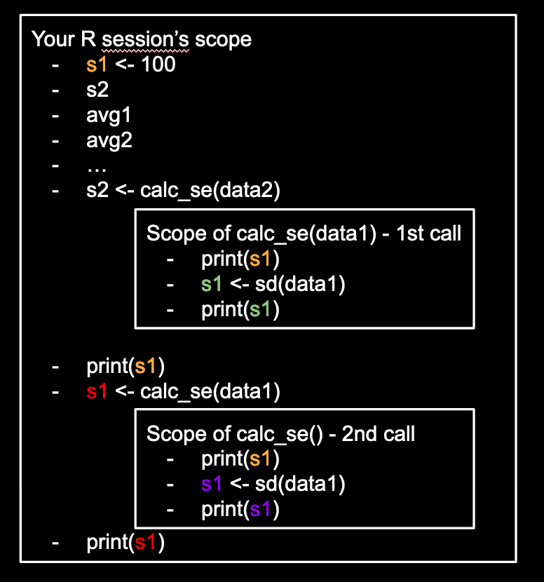
• Notice that during an assingment operation, the right hand side is evaluated first then the assignment happens.
• Notice that the two different calls to calc_se() will be in different scopes. This has implications about functions interacting with one another. In general, data is saved somewhere then different functions act on the saved data afterwards.

Exercise:

• What should happen if we re-calculate s2 <- calc_se(data2) right before test_stat is define? What would be printed?

Quick note on debugging and naming

In general, it’s not a bad practice to add print() statements at different parts of your code to make sure

• the class of the variable is what you expect (e.g. character vs numeric vs boolean when subsetting)
• the size of the data is what you expect (often people get 0 data when they expect lots of data)
• the value of the data (sometimes it’s NA without you realizing it)

Notice that this potential confusion could be avoided if we named our variables better as well. Better naming can really decrease the number of bugs in your code!