Homework 3: Simple Linear Regression

Q1 - interpreting the formulas

Please answer the following TRUE/FALSE statements according to the formulas we have shown from the simple linear regression:

• True/False, assuming \(Y>0\) and \(X>0\), the prediction formula implies that the predicted \(Y\) from regression will be above the average \(Y\) if its corresponding \(X\) value is above the average \(X\).
• True/False, assuming \(1>Corr_{(x,y)}>0\), then if a prediction for an \(X\) value that is 1 standard deviations below the average will result in a prediction \(\hat{Y}\) that is less than 1 standard deviations below the average.
• True/False, the denominator in \(r^2\) can be interpreted as the “total variability in the data relative to its average”
• True/False, the numertaor in \(r^2\) can be interpreted as the “total variability in the predictions relative to its average”
• True/False, more data, no matter what the $X$ value is, will decrease the uncertainty in \(\hat{\beta}_1\)
• True/False, the smaller the noise in our measurement, the smaller our unecrtainty in regression’s slope and intercept would be.
• True/False, with more and more data, the \(SE(Y_{new} - \hat{Y}_{new})\to 0\)

Q2 - the importance of the intercept in regression

Please generate some data as below:

n <- 50
x <- runif(n, 1, 5)
y <- 1.2 * x + rnorm(n, sd=0.4)

• Please calculate the \(r^2\) value from regression and show the code that does so. Please assume you do not know the data generation model has \(\beta_0=0\).
• Please fit the model without an intercept by specifying lm(y ~ x - 1), please show, numerically, that \(\sum_i e_i \not = 0\) in this case. Training the regression without the intercept means we are forcing \(\hat{\beta}_0=0\).
• Is the \(r^2\) higher with or without an intercept? (side note: we will show why the \(r^2\) calculation is not sensible in the future without an intercept)
• We want to understand if “fitting the intercept” can hurt. Please simulate from the true data generation process above with sim_num=10000 but fit the regression in 2 ways: with an intercept and without an intercept. Each simulation should generate 2 estimates for \(\beta_1\) (the slope parameter), one estimate with the intercept and one without. Please plot the respective histograms for the different estimates then comment which results is better?

Q3 - directionality in regression

Imagine that the data from Q2, \(x\) is actually data from a well-calibrated machine (essentially 0 error) and \(y\) is the output from an uncalibrated machine measuring the same object (noisy and potentially biased). If you were asked to use statistics to “de-bias” the machine that produced \(y\), should you fit a regression with \(y\) or \(x\) as the dependent variable (please explain!)? De-bias here means that they’ve given up on calibrating the machine that generates \(y\) and wish that your regression model will act as a second stage process to correct any systematic bias in the data. So they’ll use the uncalibrated machine to obtain biased measurements, then wish to obtain values that look like they’re calibrated.

Hint: what is the objective of the regression?

Q4 - violating the regression assumption

Please generate data as below

n <- 200
x <- runif(n, 1, 5)
y <- 0.1 + 1.2 * x + rnorm(n, sd=x)

• Which regression assumption is being violated? We will have 2 estimates for the \(SE(\hat{\beta}_1 \mid X)\):
• The first estimate is the SE from summary.lm()
• The second estimate \(SE(\hat{\beta}_1\mid X)\) is by simulating from the true data generation and fitting B=1000 different \(\hat{\beta}_{(1,j)}\) (the \(j\) index just indicate different the estimates from different simulations). Please do not overwrite your original data from above. Calculate this by simply using sd() in R over the simulated coefficients.
• Please calculate the “percent error” for each of these estimates above. Percent error is often calculated as \(\frac{\lvert new-base\rvert }{base}\). The “base” value in this problem should be \(\sqrt{\frac{1}{B} \sum[(\hat{\beta}_{(1,j)} - \beta_1]^2} \approx \sqrt{E([\hat{\beta}_{(1,j)} - \beta_1]^2\mid X)}\). Please have one sentence explaining the difference between this and the second estimate.

Q5 - Evaluating residual plots

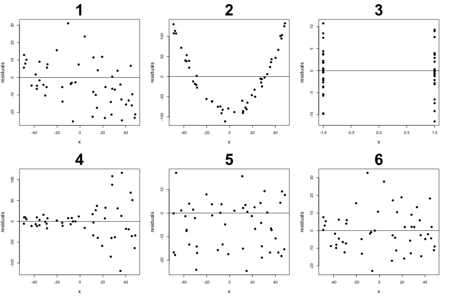
For each of the following residual plots, please comment on which of the statements cannot be rejected and explain with at most 2 sentences. Please assume the residuals are from fitting a “linear line that may not be the regression line” to the data (e.g. no curves were used to obtain residuals) and there is only one independent variable \(x\).

• the relationship between \(x\) and \(y\) linear
• \[E(\epsilon_i\mid X)=0, \forall i\]
• \[E(e_i\mid X)=0, \forall i\]
• \[Var(\epsilon_i\mid X)=\sigma^2\]
• the residual plot is from fitting a regression line (hint: if you are stuck, try to simulate data that will have residual plots as shown then fit a regression to it)

Q6 - Translating assumptions

From the paper Global Evidence on Economic Preferences:

• Which linear model assumption is being made with this quote? “Although the evidence is correlational, the previous literature has proposed various mechanisms, ranging from biological to purely social, through which gender, age, and cognitive ability might determine preferences.”
• In Table V, there are many examples of low \(R^2\) values corresponding to highly significant values. Please explain why this is possible then provide one toy simulation example that demonstrates this phenomenon.

Q7 - Counter examples

• Please create a simulation where regressing Y on X has a stronger slope, i.e. away from 0, than regressing X on Y, even though X is actually a function of Y.
• Please create a simulation where the data is from a linear model, the \(r^2\) is low, but the estimated coefficients are significantly not 0.